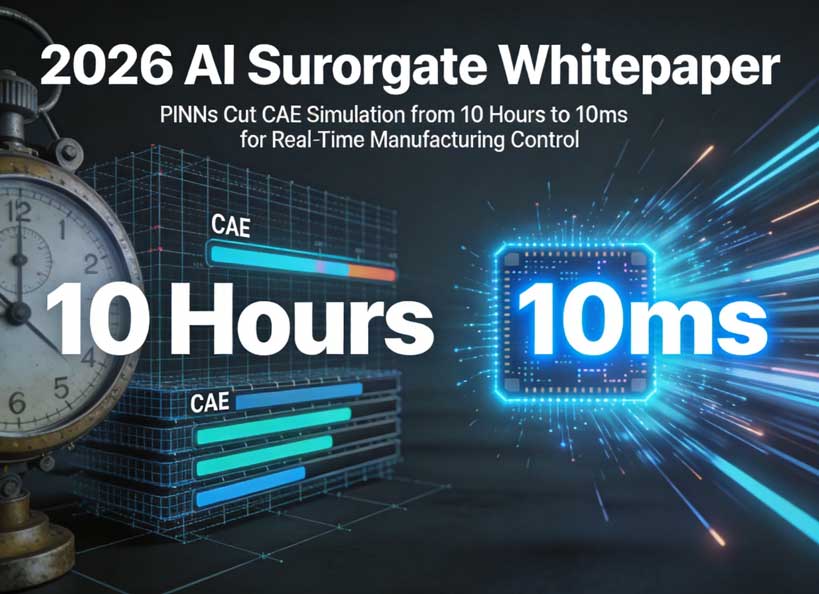
2026 AI Surrogate Whitepaper: PINNs Power Millisecond Real-Time CAE for Advanced Manufacturing
2026-09-28 15:47:00
#CEO#VP of R&D#Chief Scientist# CTO#VP of Advanced Manufacturing
Executive Summary
The most valuable intellectual property a manufacturer owns is the ability to predict physics — to know, before metal is cut or material is poured, how a process will behave. For forty years that capability has lived in computer-aided engineering (CAE): finite-element and computational-fluid-dynamics solvers that model stress, flow, heat, and solidification with remarkable fidelity. The discipline has never been more accurate. It has also never been less sufficient.
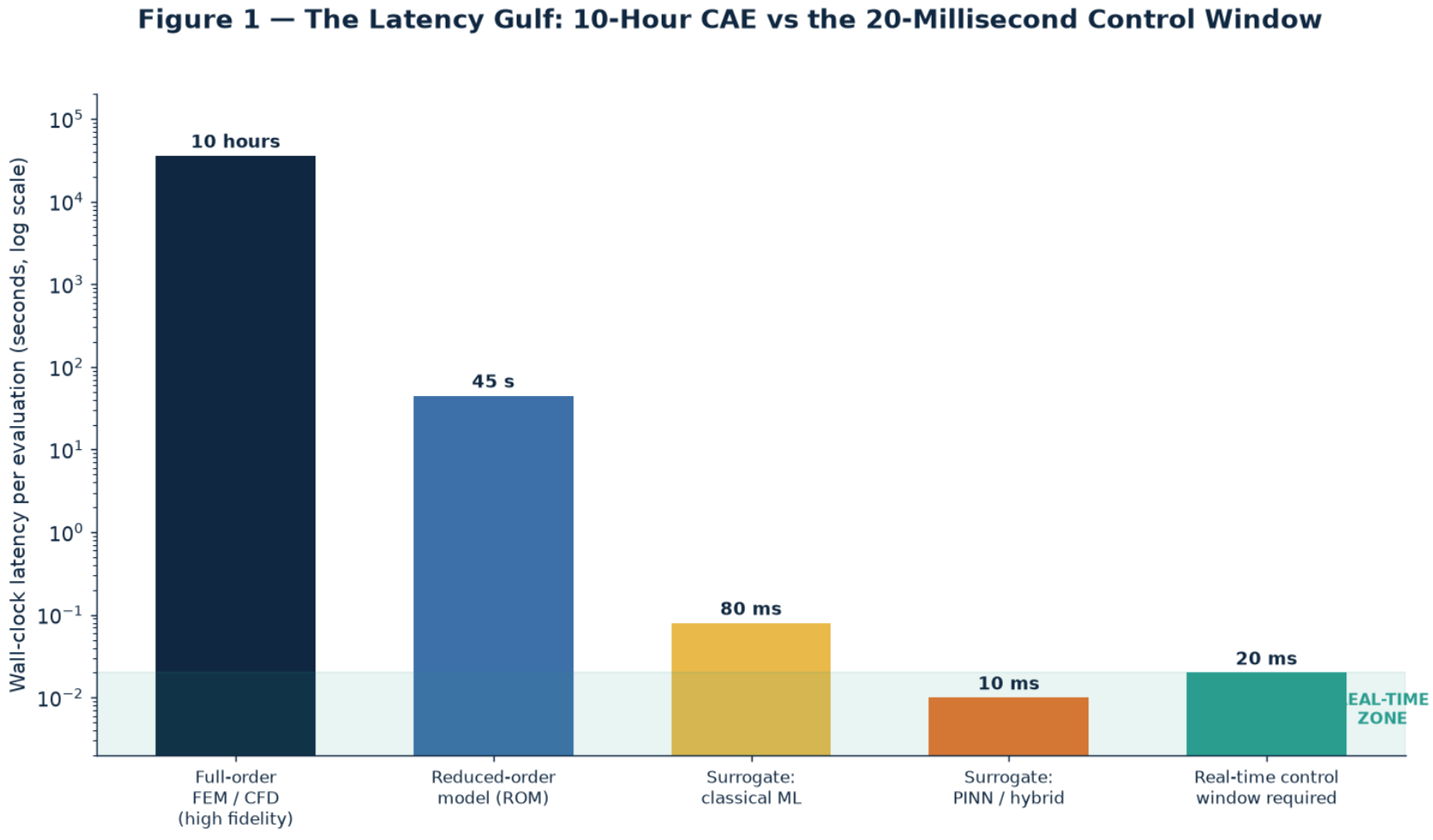
The problem is not the quality of the simulation. It is the clock. A high-fidelity model of a complex multiphysics process — a gigacasting die filling and solidifying, a laser powder-bed melt pool evolving, a reactor approaching an unstable regime — can take ten hours to solve on serious compute. The physical process it describes completes in seconds and must be controlled within a twenty-millisecond window. There is no operational universe in which a ten-hour answer steers a twenty-millisecond decision. The simulation is correct and useless at the same time.
For decades that gap was tolerable because CAE was used offline — to design a die, qualify a process, set a static recipe, and then walk away while the machine ran open-loop. In 2026 that division is collapsing under the weight of processes too fast, too variable, and too expensive to run blind. The frontier technologies every advanced manufacturer is racing to master — gigacasting, metal additive manufacturing, advanced chemicals and coatings, semiconductor processing — share a brutal property: small deviations in unseen physics become large scrap bills before any sensor-based controller can react.
The shift: from offline CAE to real-time AI surrogates
A surrogate is a model trained to approximate a slow, high-fidelity solver — or the underlying physics itself — fast enough to be queried inside the control loop. The naive version, a black-box neural network trained purely on data, is fast but dangerous in exactly the places that matter: when asked to extrapolate beyond its training data, it confidently violates conservation laws and recommends impossible states. A data-only model will interpolate smoothly and hallucinate catastrophically.
The breakthrough of the last two years is the maturity of physics-informed neural networks (PINNs) and, more importantly in production, hybrid models that embed governing equations, boundary conditions, and conservation constraints directly into learning. These models are not choosing between physics and data. They are enforcing the known physics while using data to calibrate what is uncertain — and they return answers in roughly ten milliseconds. The known laws constrain the prediction; the data calibrates the unknowns; a guardrail layer certifies whether a given run is trustworthy.
What the data shows
The Yunzhibian Solution Engine completed engineering-AI audits, surrogate builds, and TCO analyses across 360+ advanced-manufacturing and R&D sites in North America and Europe during 2025–2026. The findings behind this paper:
表格Finding Baseline Advanced manufacturers now deploying or piloting AI surrogates 65% Median high-fidelity CAE solve time for a complex multiphysics case 10 hours Real-time control window the process actually allows 20 ms First-pass scrap rate in metal additive (LPBF), median 14.2% Gigacasting first-pass scrap / reject rate, median 9.4% Share of process engineers who say offline CAE cannot steer live control 71% Sites where a black-box ML model failed because it extrapolated outside data 58% Median time to first validated surrogate insight 9 weeks
The opportunity follows the now-familiar pattern: the organizations that move deliberately convert a painful scrap and engineering-labor problem into a structural edge — better first-pass yield, dramatically faster ramp, and a real-time model of physics that compounds in value across every new product.
The reference outcome
The reference deployment in this paper — an advanced manufacturer running gigacasting and adjacent high-variability processes — replaced its offline-only, open-loop operating mode with a hybrid PINN surrogate feeding a guarded real-time controller. The board-level numbers:
This document explains exactly how the hybrid model works, why pure-data and pure-physics extremes both fail, where the deployment traps hide, and how to start within 90 days without touching a running process until the model has earned it.
How to read this whitepaper
The ten-hour simulation is not going to get faster enough to matter. Here is what does.
PART I — THE LATENCY PARADOX
1. The Best Model You Cannot Use
Walk into any advanced-manufacturing engineering group and you will find a quiet contradiction. The team is proud of its CAE capability — and rightly so. The finite-element models capture nonlinear material behavior, the CFD captures turbulent flow and heat transfer, and the correlation against physical tests is, on a good day, within a few percent. The physics is understood to a depth previous generations could not have imagined.
Ask when those models are used and the answer reveals the limit. They are used in design. They are used to qualify a process before launch. They are used, occasionally, to diagnose a failure after the fact. They are almost never used while the machine is running — because by the time the solver returns, the physical moment it described is long past. Accuracy without timeliness is documentation, not control.
2. The Two Clocks
Industrial reality runs on two clocks that do not agree:
表格Clock Typical cycle What it governs The CAE clock 10 hours per complex case (sometimes days) Design, qualification, offline analysis The process clock Milliseconds to seconds per event Filling, melting, reacting, solidifying The control clock 10–20 ms loop time Setpoint adjustment, actuation
The control loop must measure, decide, and act inside twenty milliseconds to keep a fast process on trajectory. A model that answers in ten hours is not slow by a small margin; it is slower by a factor of roughly 1.8 million. No amount of overnight batch scheduling, no bigger cluster, no cloud burst of GPUs closes a six-orders-of-magnitude gap for a decision that exists only in the present instant. The CAE model describes the process the way a history book describes a battle — accurately, and far too late to command it.
3. Why Faster Hardware Does Not Save CAE
It is tempting to assume that continuing hardware progress will eventually make full-order models real-time. It will not, for a structural reason: as compute gets cheaper, engineers use the budget to add fidelity, not merely to run the same model faster. Mesh refinement, additional coupled physics, finer time-stepping, and uncertainty quantification absorb the gains. The ten-hour case of today is the answer to yesterday's question on yesterday's hardware; tomorrow's model, run on tomorrow's hardware, will still take hours because ambition scales with capability.
Meanwhile the control window is fixed by physics and hardware — a melt pool does not slow down because computers got faster. The gap is therefore not a temporary technology lag awaiting Moore's law. It is structural, which is why it requires a different kind of model rather than a faster version of the same one.
4. The Offline Compromise That Worked — Until Now
The historical resolution was a clean division of labor. CAE lived entirely offline. Engineers used it to design the die, optimize the geometry, and derive a fixed recipe — the temperatures, speeds, and pressures the machine would use. That recipe was then loaded into the controller, which ran the process open-loop or with simple sensor feedback, while the CAE model stayed in the engineering department. The slow model set the starting conditions; the fast but physics-blind controller handled execution.
This compromise worked reasonably for stable, well-understood, high-volume processes. It fails when the process is intrinsically variable batch to batch, when the physics is too complex to capture in a fixed recipe, or when the cost of being wrong is high — precisely the characteristics of the frontier processes defining competitive advantage in 2026.
5. Why Sensors Are Not Enough
The reflexive answer — add more and faster sensors — also has a limit. Sensors measure what is happening at a point, but they do not reveal the full internal state of the physics. A thermocouple reads temperature at one location in a die; it does not reveal the evolving solidification front, the residual stress accumulating, or the defect forming a centimeter away. By the time a downstream symptom is measurable, the defect is already created. A sensor can report a problem faster than a ten-hour model, but it cannot infer the unseen field variables that cause it.
What control actually needs is an estimate of the complete physical state, now — internal temperature fields, flow, phase, stress — from sparse sensor readings. That is state estimation of a complex distributed system, and it cannot be done by sensors alone or by a ten-hour solver. It requires a fast model of the physics, which is exactly the role of a surrogate.
6. The Paradox Stated
The latency paradox is therefore sharp and simple. The manufacturers with the best physics models are often the ones least able to use them where value is now created — at the instant of production. They possess deep offline understanding and operate in real-time ignorance of the very fields they can model. The strategic asset is locked in the wrong time domain.
The resolution is not to abandon the high-fidelity model but to distill it — to train a fast approximation that preserves the essential physics and can be queried inside the loop. Done naively, that distillation produces a dangerous black box. Done with physics embedded and validation enforced, it produces something genuinely new: real-time access to the physics the organization already understands offline.
PART II — THE PHYSICS-SCRAP TAX
7. Where the Money Leaves
The cost of running complex physics blind is not theoretical; it appears on the factory floor as scrap, rework, and ramp delay. The frontier processes that most need real-time physics are also the ones with the least forgiving economics — expensive material, high energy, long cycle times, and defects detected only after the part is complete.
8. Gigacasting — Defects Hidden in a 90-Kilogram Part
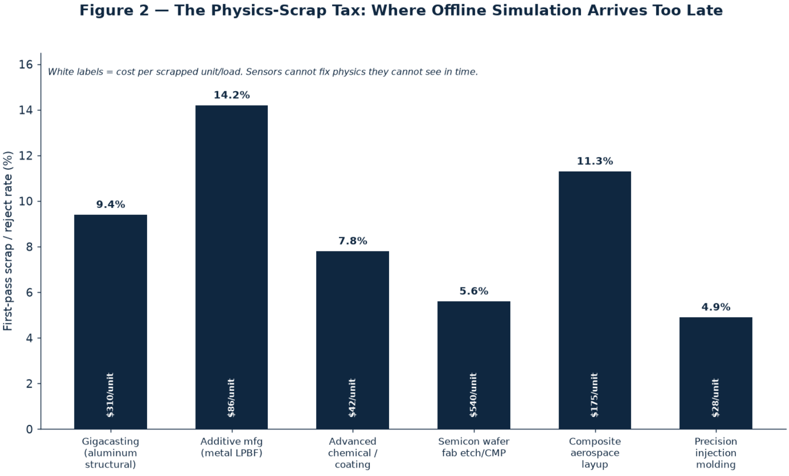
Gigacasting replaces dozens of stamped and welded components with a single large aluminum structural casting. The economic logic is compelling; the physics is ferocious. Molten aluminum must fill a die the size of a small car before solidification fronts close off flow, and the resulting part must avoid porosity, cold shuts, and distortion while cooling. First-pass scrap in our dataset ran at a median 9.4% , and each rejected casting represents not only the metal but a large heat-treat and machining investment already sunk.
Worst of all, many defects are internal and invisible until later inspection or, in the worst cases, after the part is in a vehicle. A fixed recipe cannot compensate for the variability that actually occurs — differences in melt temperature, die thermal state from the previous shot, and alloy chemistry. Real-time adjustment of the shot profile based on the evolving fill state is the difference between 9% scrap and 4% scrap — and a ten-hour simulation cannot provide it shot by shot.
9. Metal Additive — The 14% Frontier
Laser powder-bed fusion offers geometry nothing else can achieve and carries the highest first-pass failure rate of the major processes — a median 14.2% , higher in difficult alloys. A part that builds for days can be ruined in one layer by a melt-pool instability, lack-of-fusion defect, or residual-stress warp. The defect often exists long before it is detectable. A fixed set of laser parameters cannot respond to the local thermal history, which varies across geometry, height, and cooling.
What LPBF needs is continuous, millisecond-scale control of laser power and speed based on the estimated melt-pool state — a textbook surrogate application, because full simulation of the evolving thermal field is intractable in real time and sensors see only the surface.
10. Advanced Chemicals, Coatings, and Wafers
The pattern repeats across process industries. Advanced coating and chemical processes depend on reaction and transport phenomena that drift with feedstock and ambient conditions; a 7.8% median reject rate understates the batch cost when an entire reactor load is lost. Semiconductor processing — etch and chemical-mechanical planarization — runs at a lower median scrap of 5.6% but at the highest cost per scrapped unit (roughly $540), where even a small drift across a wafer batch is extremely expensive and the physics at the wafer surface cannot be directly observed.
In each case the controlling variable is an internal field — concentration, reaction rate, etch rate distribution — that a fast physics model can estimate and a sensor alone cannot see.
11. The Ramp Tax
Scrap is only the visible cost. A second, often larger penalty is paid during new-product introduction. When a process is qualified using offline CAE and then tuned on the machine through trial and error, achieving stable yield can take months and thousands of scrapped parts. Every new geometry, alloy, or die restarts the learning loop because the knowledge lives in a static recipe rather than in a predictive model.
Organizations with a real-time surrogate compress this brutally: the model generalizes across designs because it encodes physics, so a new product starts from a predicted optimal trajectory rather than from scratch. The competitive consequence — weeks versus months to stable production — is frequently worth more than the scrap savings themselves.
12. The Engineering-Labor Drag
A third cost is the scarce engineering talent trapped in a slow loop. Process engineers run a CAE case, wait hours, inspect, adjust, resubmit, wait again. A single optimization can consume weeks of calendar time and a great deal of expert attention that could instead be applied to higher-value problems. The ten-hour clock is not merely a control problem; it is a throughput constraint on the most valuable people in the organization.
A fast surrogate flips the ratio: engineers query thousands of scenarios interactively, optimize against the model, and reserve the slow high-fidelity solver for final confirmation. The same expert team accomplishes dramatically more — which is why the surrogate's return appears in engineering-labor metrics as well as in yield.
13. The Tax, Totaled
Across scrap, ramp delay, and engineering labor, running complex physics on the offline/open-loop model is a large and recurring tax — and one that rises as manufacturers pursue exactly the difficult, physics-intensive processes that define the frontier. The do-nothing position is not stasis; it is a compounding disadvantage as more advanced competitors compress the same loops.
The strategic question is no longer whether a faster path to physics is desirable. It is whether the fast model can be made trustworthy — accurate where data is abundant, constrained by physics where it is not, and honest about when it should not be believed. That question defines the rest of this paper.
PART III — THE FIVE FAILURE MODES
14. Failure Mode I: The Black-Box Trap
The first and most common failure is treating an ordinary supervised neural network as sufficient. Train a flexible model on simulation or process data, the reasoning goes, and it will learn the physics implicitly. Within the range of its training data it often does — interpolate between known cases and a black box can be remarkably accurate and very fast. The failure arrives exactly at the boundary of what it has seen.
Asked to extrapolate — a new geometry, an unusual material, an extreme operating point — the black box has no notion that outputs must obey conservation, remain positive, or stay bounded. It produces smooth, confident answers that are physically impossible, and it does so without any warning flag. 58% of sites in our dataset saw a black-box ML model fail specifically through out-of-distribution extrapolation. In a control loop that is not an accuracy problem; it is a route to a crashed machine or a scrapped batch. The first rule of surrogate design is therefore: never let an unconstrained model act where it has not got physics to hold it.
15. Failure Mode II: The "PINN Solves Everything" Reflex
The mirror failure is assuming that simply rebranding a network as a PINN guarantees success. Embedding a PDE residual into the loss is a powerful idea, but it is not magic. PINNs are notoriously sensitive to optimization: loss-term weighting, collocation-point sampling, and stiffness can make training difficult, and for some well-conditioned problems a PINN is both harder to train and less accurate than a simpler approach. PINNs also still depend on the correctness of the governing equations and boundary conditions — encode the wrong physics and the network faithfully converges to the wrong answer with high confidence.
The mature stance treats the PINN as one tool on a spectrum rather than a universal answer, and in most real production systems it appears inside a hybrid architecture (Part IV) combined with a reduced-order model and data — not as a standalone slogan. Discipline in where physics-informed learning is genuinely warranted is what separates working deployments from impressive demos that never stabilize.
16. Failure Mode III: The Simulation-Reality Gap
The third failure is training surrogates on CAE output alone and deploying them against the real process. A high-fidelity model is an approximation of reality, not reality; it omits effects, idealizes boundary conditions, and depends on assumed parameters. A surrogate trained only on simulation learns the model's biases as if they were truth, and when asked to steer the actual machine it inherits a systematic gap — sometimes precisely in the regimes that matter for scrap.
The remedy is pairing: synchronizing simulation labels with real sensor traces and including the discrepancy as part of what the model learns. The strongest systems use simulation to provide dense, cheap labels and real data to correct the offset, so the surrogate tracks the physical machine rather than an idealized picture of it. Skipping this step produces a model that validates perfectly against the solver and fails on the floor.
17. Failure Mode IV: The Validation Void
The fourth failure is deploying without a defensible answer to the question "when should the model not be believed?" A surrogate will, inevitably, encounter inputs unlike its training data. If nothing detects that condition, the controller follows a confident guess into a new regime. Organizations that succeed build an explicit guardrail layer: an uncertainty estimate per output, an in-distribution check on the inputs, and a physics-consistency test on the prediction — with a defined safe fallback (hold the last good setpoint, rever
解锁后续 88% 内容Unlock the Remaining 88% of Evaluations & the Decision Engine
The second half includes: a core solution cross-comparison matrix, a key parameter selection checklist, an implementation pitfalls guide, and a TCO & ROI calculator for mainstream approaches.
Get Your Custom Solution (View in Dashboard)